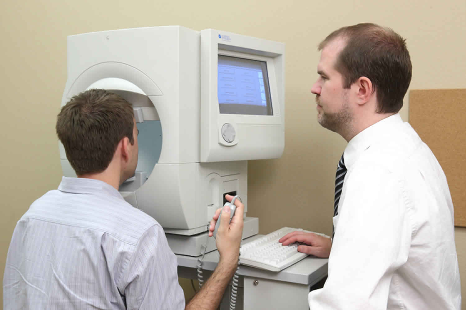
What is a visual field test

Visual field test looks for visual field defects and their location. Central and peripheral vision is tested by using visual field tests. Careful detection of visual field defects can be diagnostic of many eye and/or neurological conditions, including glaucoma or retinitis pigmentosa. In glaucoma – as well as other conditions – it is vital to repeat visual field testing to track any changes over time.

Examining visual fields is an integral part of a full ophthalmic evaluation. Several methods for assessing visual field loss are available, and the choice of which to use depends on the patient’s age, health, visual acuity, ability to concentrate, and socio-economic status. Available techniques can test the full field (including confrontation, tangent screen, Goldmann perimetry and automated perimetry), or assess just the central field of vision, such as the Amsler Grid.

The Visual Field Interpretation ¹:

These guidelines must be followed in this order for the most accurate results.

1. Look for signs of unreliable fields: Are there many false positives (> 15% using SITA), or losses of fixation (> 33%)? Is there a lens rim artifact or uncorrected ptosis? If the fields appear reliable, continue to step 2.
2. Look at the sensitivity map to determine whether the field is within normal limits. If the fields are within normal limits, there is no further analysis. If one or both of the eyes exhibit abnormal fields, continue to step 3.
3. Is the visual field damage present in one or both eyes? If only one eye is affected, the damage is located in front of the optic chiasm (i.e. the cornea, vitreous, retina, or optic nerve of only one eye). Damage in the visual fields of both eyes could be due to damage at the level of the optic chiasm and beyond, or due to separate damage in the visual pathways of each eye anterior to the chiasm.
4. Locate the region of the visual field deficit. Refer to the patterns of visual field defects chart to determine the likely region of damage to the visual pathway.
5. Identify the shape of the visual field defect. Refer to the chart to determine the likely region of damage to the visual pathway.
6. Compare these visual fields with each of the patient’s previous visual field tests to identify progression of visual field loss. Do not take a shortcut by comparing these fields to only the most recent visual field, as this may be misleading. Generally six or more visual field tests are necessary to evaluate disease progression. Consider the findings in the context of the physical exam findings and the results of other tests and imaging.
7. If there is uncertainty, consult with colleagues.

The Visual Field

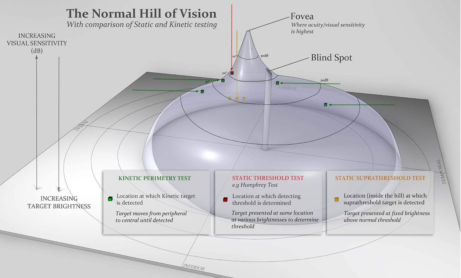
The normal eye can detect stimuli over a 120º range vertically and a nearly 160 degree range horizontally. From the point of fixation, stimuli can typically be detected 60º superiorly, 70º inferiorly, 60º nasally, and 100 degrees temporally (laterally) ², though the true extent of the visual field depends on several features of the stimulus (size, brightness, motion) as well as the background conditions. Under normal daylight (photopic) conditions, the smallest or least intense visible objects are only seen in the central region of the visual field. The field of vision is often depicted as a three dimensional hill, with the peak sensitivity to stimuli occurring at the point of fixation under photopic conditions, decreasing rapidly in the 10º around fixation, and then decreasing very gradually for locations further in the periphery ³. Nerve fibers pass through the sclera at the optic nerve head, typically 10-15º nasal to fixation. At this location, no photoreceptors are present, creating a normal absolute scotoma ⁴. A physiologic scotoma (a blind spot) exists at 15° temporally where the optic nerve leaves the eye. Definitive location varies slightly on an individual basis. The average blind spot is 7.5° in diameter, vertically centered 1.5° below the horizontal meridian ⁴. See Figure 1. For dim night lighting (scotopic) conditions, the mid periphery is the most sensitive region of the visual field.

Several basic conditions must be met for a successful map of the visual field to be produced by any method. The individual must be able to maintain a constant gaze toward a fixed location for several minutes. Each eye is tested separately while the opposite eye is covered with a patch. Refractive correction must be made with a test lens. Spectacles must not be worn because they can cause false defects in the visual field due to their shape ⁵. In addition, correction must be made for presbyopia, to reduce accommodative strain. Standard adjustments for presbyopia are available based on age alone. To correct an astigmatism >0.75 diopters, a cylindrical lens must be used. If the eyelid or lashes obstruct the visual axis, the lid may be taped to the forehead to lift it out of the way.

Figure 1. Normal visual field (left eye)

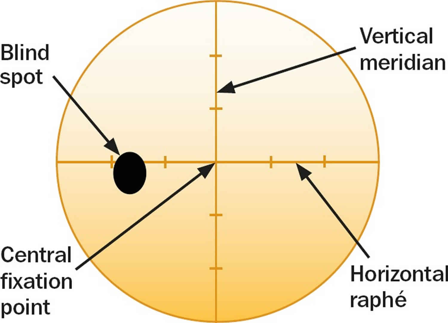
Figure 2. Normal hill of vision

Confrontation visual field test

The first thing you should do is to ask if the patient has noticed a visual field defect. The problem with this approach alone is that early (or even moderate) visual field defects often go unnoticed, particularly if only one eye is affected.

Useful questions to ask are:

• Have you noticed if any part of your vision is missing in either eye? Have you noticed any gaps in your vision?
• If you close each eye in turn, does what you see differ from one eye to the other?

In addition, it is essential to enquire about past ophthalmic and medical history, concentrating on family history, dietary/ drug/smoking/alcohol history, and whether there are any additional ophthalmic or neurological symptoms.

Visual field testing using confrontation only takes a few minutes, and should be mastered by all eye care workers, since it can provide a lot of useful information. Initially it is best to try and detect gross (absolute) defects. Position yourself in front of the patient, facing her/him with your face level with that of her/his, at a distance of about a metre. A comparison of examiner and patient fields is made, the assumption being that you, as the examiner, have normal visual fields (this is another reason why you should undergo visual field testing yourself).

First test the binocular visual field and then test each eye separately. A defect is detected by the absence of a patient response to the showing of a target, when the target is visible to you.

Testing to confrontation with both eyes open

1. Ask the patient to stare directly and steadily into your eyes. Staring can cause embarrassment or awkwardness, so allow the patient to rest and try again if they find it difficult to look at you so directly. Check that the patient can look steadily at your eyes while you look steadily at theirs. Ask the patient whether any part of your face is missing or indistinct.
2. Check the patient’s left hemi-field by making a fist with your right hand and holding it in their left hemi-field, at eye level, just to the right of your face. Making sure that the patient is still holding your gaze, raise one to four fingers and ask how many fingers can be seen. To test the upper and lower quadrants, move your hand up and to the right, and down and to the right, repeating the test at various points. This simple finger-counting test is particularly useful for detecting visual field loss due to neurological problems (such as strokes), but is only useful for patients with glaucoma when the visual field loss is severe.
3. To test the patient’s right hemi-field and upper and lower quadrants, repeat the finger-counting test using your left hand, starting just to the left of your face and moving up and left and then down and left.
4. A useful, additional test to perform in patients with a suspected homonymous hemianopsia (i.e. loss of either the right or left field of vision in both eyes, often from a stroke) is to test for sensory inattention. Hold both hands up and wiggle the fingers of the right hand, followed by those of the left hand in each hemi-field. If the patient sees the moving fingers, then wiggle one finger of each hand at the same time – if the patient can only see movement on one side then they may have a subtle hemianopia.

Testing each eye to confrontation

1. Ask the patient to cover their own eye with the palm of their hand (not their fingers, as it is easy to peep between fingers). Remember that you should close your eyes in turn too, so that you are comparing the field in your right eye with the field of the patient’s left eye.
2. Do the finger counting test first (static testing). Be sure to test on both the left and the right for each eye tested.
3. Next, bring your target finger from the far periphery in towards the central region (kinetic testing). Ask the patient to say when they first see the target. Repeat from several different directions, ensuring that the full 360° for each eye is tested. The examiner should remember to perform kinetic testing at a speed appropriate for the patient’s responses.
4. Next, test the peripheral field with a white-headed neurological pin (beyond a central 30° radius) and the central field with a red-headed neurological pin (within a 30° radius). Testing with neurological pin targets gives much more accurate results than testing with fingers, and can detect earlier visual field loss. Red-headed neurological pins are also useful for assessing the size of the blind spot (e.g., with papilloedema), again by comparing the size of your blind spot with that of the patient’s. In addition, red-headed neurological pins can be used to test for red-desaturation in early optic nerve disease.

Goldmann visual field test

Goldmann visual field perimetry is not as widely available as Humphrey visual field because it requires skilled perimetrists who manually map the visual field without the aid of a computer algorithm. Light is projected into a white bowl with a standardized background light intensity. The projected light forms a fairly circular stimulus. Six stimulus sizes are available, ranging from 0.0625 mm² (about 6 minutes of arc diameter) to 64 mm² (about 2 degrees in diameter) when viewed at 30 cm, which is the standard distance between the patient’s eye and the stimulus on the background. The overall field mapping technique used is a form of kinetic perimetry, where a stimulus is moved into the field of vision.

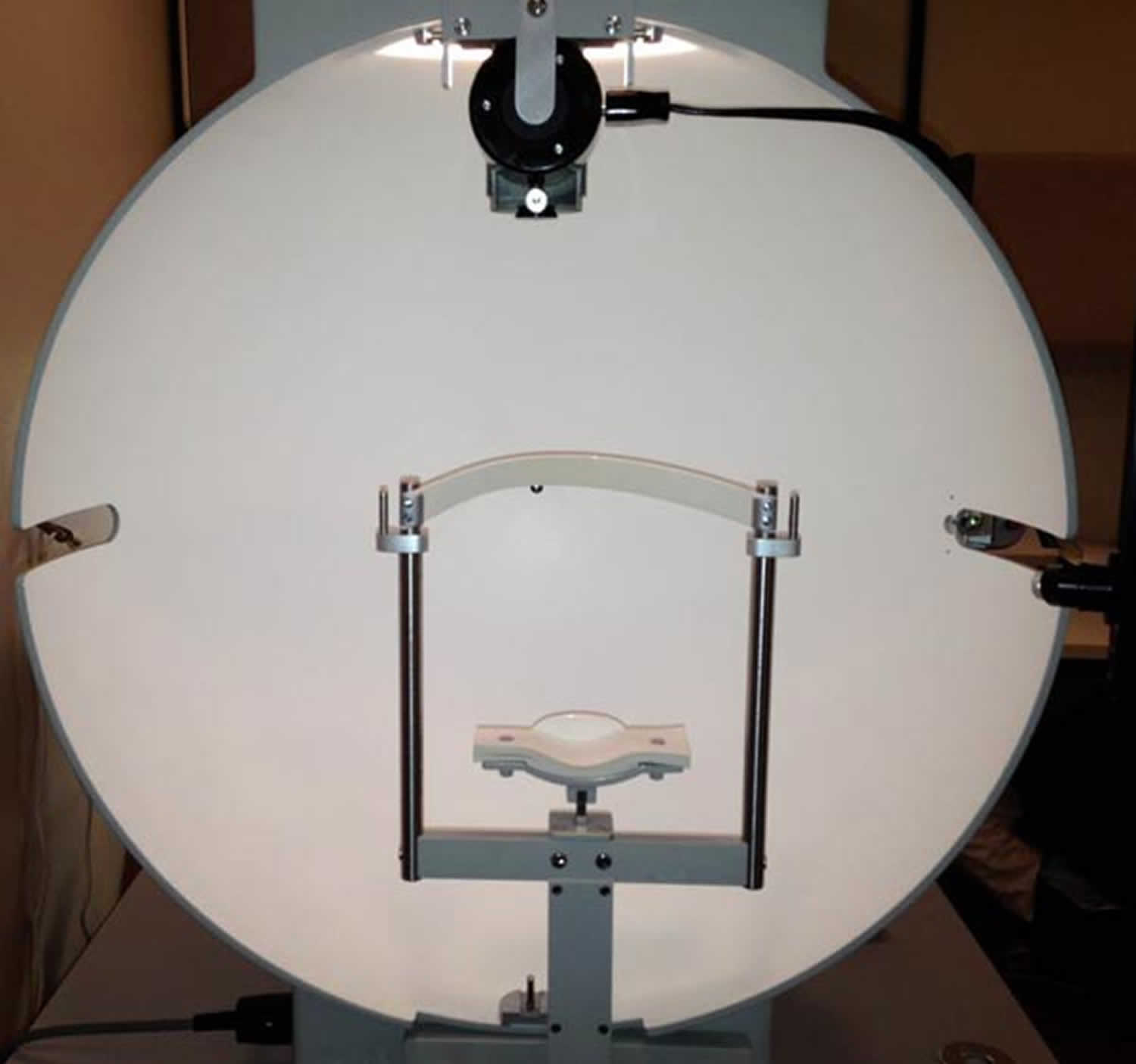
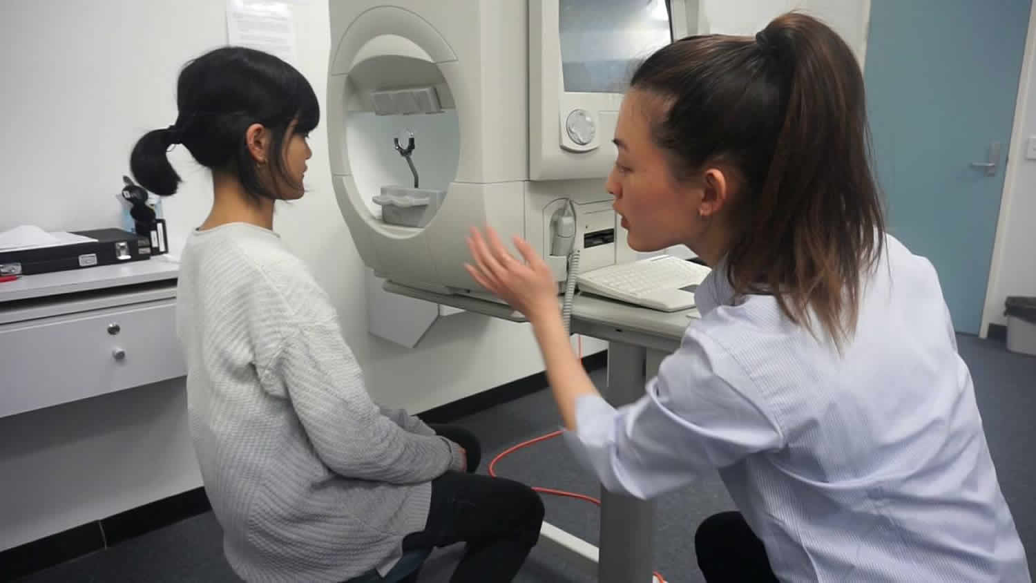
During a Goldmann field test, the patient positions their eye opposite the center of a white hemispherical bowl (Figure 3). The patient fixates upon the central target 33 cm away, while the examiner sits opposite viewing through an eyepiece to ensure good fixation throughout the test. The examiner moves an illuminated white target from the periphery towards the center, and the patient presses a buzzer to indicate when they first see the target. This is repeated from different directions —allowing the examiner to plot the patient’s field of vision—using targets varying in size and brightness. The examiner plots the blind spot and the edges of scotomas in a similar way, with the patient pressing the buzzer to indicate when they first see the light target moving from a blind to a seeing area. The examiner also performs static testing—involving the brief appearance of the stationary light target—in the four quadrants within the central 20° or so, marking a tick on the chart when the patient sees the target and a cross if they do not.

The target sizes are labelled with three alphanumeric digits, for example, ‘V4e’.

1. The first digit is a Roman numeral (I–V), indicating the size of the target, for example, V is equivalent to a target diameter of 9.03 mm. With every drop in number (eg, from V to IV) the diameter halves.
2. The second digit is an Arabic number (1–4), indicating the brightness of the stimulus: the larger the number the higher the luminance.
3. The third digit is a letter (a–e), indicating a finer calibration of luminance. ‘4e’ is equivalent to 10-decibel (dB) brightness; each consecutive drop in number represents a 5 dB change and each drop in letter represents a 1 dB change.

By convention, the examiner maps three isopters: lines of equal sensitivity to targets of a specified size and luminance. The first isopter, mapping the farthest peripheral vision, requires the largest and brightest target ‘V4e’. Another isopter is mapped in the central 30° of vision, and a third isopter is intermediate between these two. The isopter lines therefore show the margins of different visual sensitivity, analogous to the contour lines of a map marking different elevations. This allows us to visualize the hill of vision (Figure 2). The base of the hill represents the area at the periphery with least visual sensitivity, detecting only the largest and brightest target. As you move up towards the peak of the hill, the visual sensitivity increases and the patient sees smaller and dimmer targets.

Figure 3. Goldmann visual field test

Goldmann visual field test results interpretation

The final result of a Goldmann visual field test is a diagram similar to a topographic map. An analogy commonly used to conceptualize these diagrams is the “island of vision.” In this analogy, the visual field is an island with a central peak and the altitude correlates with the visual sensitivity in a given location. In this analogy, physiologic blind spot is represented by a pit or a well in the island. The isopters are named with three characters: a Roman numeral, an Arabic number, and a letter. The Roman numeral indicates the Goldmann size of the stimulus. The Arabic number and letter indicate the attenuation of the light. The combination “4e” is used when there is no attenuation. For each Arabic number less than “4,” the light is attenuated by 5 dB. For each letter earlier in the alphabet than “e,” the light is attenuated by 1 dB. Within the confines of an isopter, the patient is able to see a light of this size and intensity. Scotomata are represented by areas shaded with a solid color. The color represents the depth of the scotoma, or the dimmest, smallest stimulus the patient is unable to see in that area. For example, in the image below, the physiologic blind spot is shaded orange like the I2e isopter. This suggests the patient is unable to see the I2e stimulus in the area but was able to see the dimmer I4e stimulus.

Interpreting the Goldmann visual field test

The key to interpreting Goldmann visual fields is to keep in mind the normal hill of vision (Figure 2) and how it compares with the patient’s results. The skill is in identifying patterns and observing any change with repeated tests. This may require experience to be adept, though the following checklist may help (Figure 4):

1. Patient name and date of test: a good habit always to check the test belongs to your patient.
2. What is the largest peripheral field (V4e)? This can vary according to age and test response. It normally extends to approximately 60° nasally, 90° temporally, 60° superiorly and 70° inferiorly. Thus, the superior aspect of the field is usually less sensitive than the inferior field, though ptosis could also artefactually reduce it.
3. Is there any distortion to the ‘contours’? (Contours are the smaller isopters corresponding to targets that are either smaller or dimmer or both).
   • A. Is the isopter smooth, as expected for a normal hill of vision?
   • B. Is there restriction? Examples would be a nasal step in papilloedema or an altitudinal defect in anterior ischaemic optic neuropathy.
   • C. Are the isopters spaced, as expected for the normal hill of vision?
     • (1) A tiny central field with ‘stacked’ isopters—very close to one another as in a steep hill—usually denotes functional overlay; however, patients with genuine retinal and striate cortex lesions may also have stacked isopters.
     • (2) Isopter lines that cross always indicate unreliable test: isopters cannot cross since this would indicate two different sensitivities at one location.
     • (3) Spiralling isopters suggest functional visual loss and indicate a steady decline in sensitivity during the test.
   • D. Are there scotomas? It is important to correlate this with the patient’s symptoms and clinical (bedside) examination.
4. Is the blind spot size enlarged? This is particularly relevant in papilloedema. The normal blind spot size is oval, roughly 10° in diameter, and located 10–20°
   temporally from the central fixation point.
5. Is the central field affected? Was static testing done (indicated with a tick when the patient saw the target)?
6. Is any defect monocular or binocular, when comparing the fields for each eye? If binocular, is the defect homonymous or heteronymous?

Any comments written about patient fixation or attention also help.

• Small pupil size, ptosis and incorrect positioning of a correcting lens may affect the peripheral field.
• Inadequate correction of refraction error for the viewing distance (33 cm) may affect the central field.

Figure 4. Goldmann visual field test results interpretation

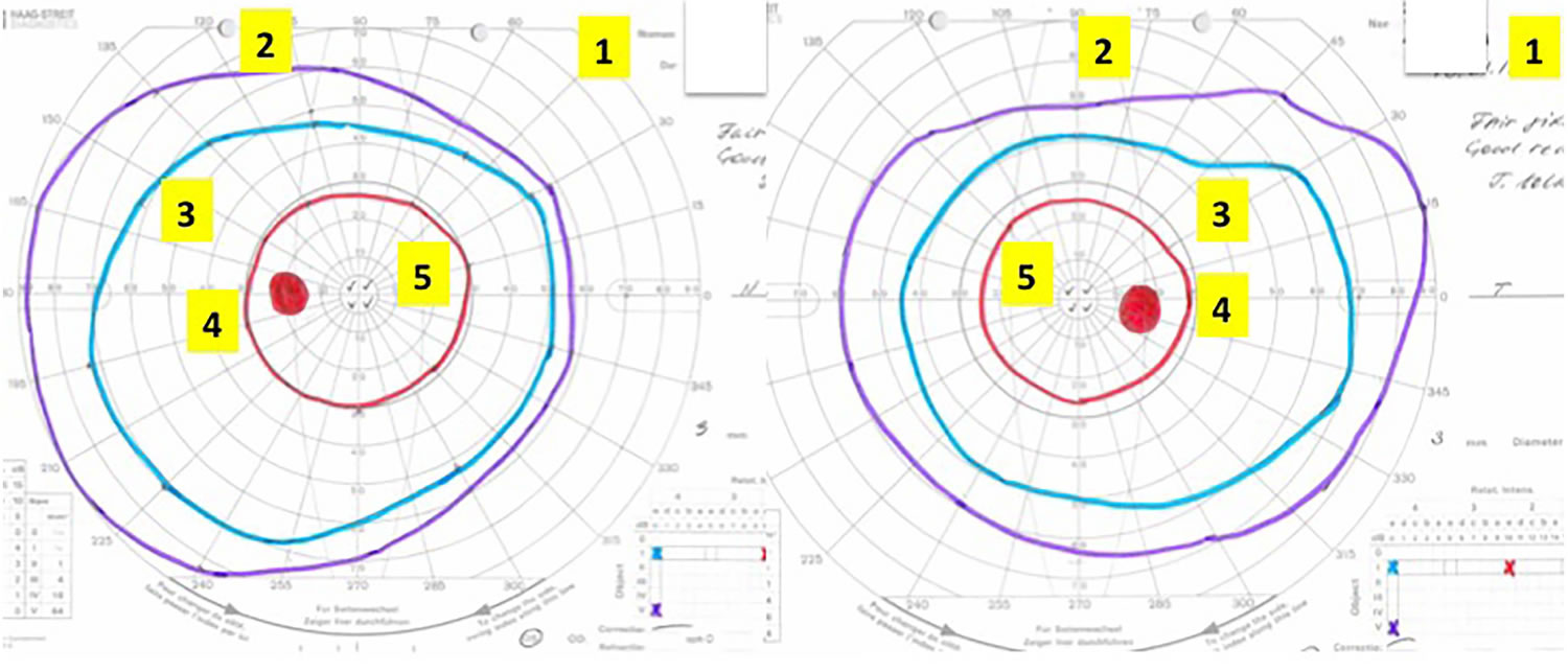
Footnote: Interpreting the Goldmann visual field.The chart is viewed from the perspective of the patient looking into the test bowl, as if patient is looking into the paper. Suggested checklist to review the Goldmann fields systematically (see text for details):

• 1. Patient name and identification number, date of test.
• 2. The largest isopter, that is, peripheral field.
• 3. The other isopters—any distortion to the ‘contours’ of the hill of vision? Any scotomas?
• 4. Blind spot.
• 5. Central vision.
• 6. If there is an abnormality, is it monocular or binocular? If binocular, is it homonymous or heteronymous?
• 7. Other, for example, comments about fixation or attention.

This is an example of normal Goldmann fields. In contrast, this patient did not perform well on the Humphrey visual fields, with poor reliability and cloverleaf pattern (Figure 6).

Humphrey visual field test

The same principles apply to the Humphrey visual field test as to the Goldmann visual field test, but instead with static light stimulation. The machine can also be programmed to perform kinetic tests. The illuminated targets appear for 200 ms at predetermined locations on a grid. Humphrey visual field tests are widely used in glaucoma clinics, the most common set up being to test the central 24° (‘24-2’ setting). Some examiners test smaller or wider visual angles; however, the wider the visual angle tested, the more coarse the grid, and hence the greater the likelihood of missing small scotomas. The 24-2 assesses the central 24° with a 54-point grid; 10-2 assesses the central 10° with a 68-point grid; and 30-2 assesses the central 30° with a 76-point grid.

During Humphrey Visual Field testing, the patient places his head in the chinrest and fixes his gaze toward a central fixation point in a large, white bowl. As stated above, this test is an example of static perimetry. It assesses the ability to see a non-mobile stimulus which remains for a brief moment (200 ms) in the visual field. When the patient sees a presented stimulus, he presses the button on a handheld remote control. Different locations within a given region of the visual field are tested until the threshold, or the stimulus intensity seen 50% of the time, is seen at each test location.

Stimuli vary in size and luminous intensity. Goldmann size III (about ½ degree in diameter) is generally used, but Goldmann size V (approximately 2 degrees in diameter) is available for patients with decreased visual acuity (< 20/200) or other visual impairment. Goldmann sizes I, II, and III are rarely used clinically. The luminous intensity of the stimuli can be varied over a range of 0.08 to 10,000 apostilbs (asb). It is reported in decibels (dB) of attenuation, or dimming, extending from 0 dB (the brightest, unattenuated stimulus) to 51 dB (the dimmest, maximally attenuated stimulus). If the patient is unable to see even the brightest, unattenuated stimlulus, it is reported as <0 dB.

The Swedish Interactive Thresholding Algorithm (SITA) is frequently used. SITA is a forecasting procedure that uses Bayesian statistical properties that is similar to the methods used for providing weather information and predictions. SITA allows for more rapid analysis than would be possible without forecasting. By taking into account a user’s results in nearby locations, stimuli that are unlikely to be seen, or extremely likely to be seen are not tested exhaustively. Instead the stimuli that are likely near threshold are tested.

Figure 5. Humphrey visual field test 

Humphrey visual field test results interpretation

All of the information provided on the Humphrey Visual Field test printout is important. Patient identity information and the specific test and stimulus size are located near the top of the analysis. It is important to verify that the patient’s birthdate was properly entered as an error will result in comparisons with normals in the wrong age group.

Beneath the patient’s name is a statement giving information about the testing parameters, such as “Central 24-2 Threshold Test.” The first statement, “Central 24” indicates that the central 24 degrees of visual field were analyzed. The next number indicates how the grid of points is aligned to the visual axis. The number “1” indicates that the middle points are overlying the horizontal and vertical meridians. The number “2” indicates that the grid of points straddles these meridians. This is the setting most commonly used, as it is easier to assess whether visual field defects respect the horizontal or vertical midline.

Next on the report are the reliability indices, including fixation losses, false positives, and false negatives. Fixation losses occur when the patient reports seeing a stimulus that is presented in the predicted area of the physiologic blind spot. False positives occur when a patient presses the button when no stimulus is presented. Eager-to-please participants sometimes struggle with high false positive rates (i.e., they are “trigger happy”). False positives can often be corrected by providing a simple statement that many stimuli will not be seen even with normal vision. False negatives occur when a patient fails to see a significantly brighter stimulus at a location than was previously seen. False negatives are usually the result of attention lapses or fatigue and are difficult to correct.

The visual threshold is the intensity of stimulus seen 50% of the time at each location. The threshold values of each tested point are listed in decibels in the sensitivity plot. Higher numbers mean the patient was able to see a more attenuated light, and thus has more sensitive vision at that location. To the right of the numerical sensitivity plot is the grayscale map. This map presents sensitivity across the patient’s visual field with lighter regions indicating higher sensitivity and darker regions reflecting lower sensitivity. The sensitivities are not compared to any normative database. Therefore the map may draw attention to an irregularity within a field, but may minimize field loss if loss is more homogenous across the field. Caution should be used as it can be misleading based on where the machine chooses to make the cutoff between the different shades of gray. The raw threshold data should always be assessed in conjunction with the grayscale representation.

The numerical total deviation map compares the patient’s visual sensitivity to an average normal individual of the same age. It is useful to compare with age-matched normal thresholds as sensitivity normally decreases gradually with age. Positive values represent areas of the field where the patient can see dimmer stimuli than the average individual of that age. Negative values represent decreased sensitivity from normal.

The numerical pattern deviation map shows discrepancies within a patient’s visual field by correcting for generalized decreases in visual sensitivity. It is useful to show localized areas of sensitivity loss hidden within a field that is diffusely depressed. For example, a person with dense cataracts may have decreased threshold across the entire visual field and this may obscure more focal losses due to coexisting disorders like glaucoma. Rather than comparing the patient’s threshold values with a normative database, the pattern deviation analysis finds the patient’s 7th most sensitive (85th percentile) non-edge point and gives it a value of zero ⁵. Each other test location is then compared with this value to correct for any generalized depression. It has been demonstrated that this method is the best for separating widespread or diffuse loss from localized loss.

The bottom-most probability plots are grayscale versions of the total deviation and pattern deviation maps. These maps may be useful to visually represent the statistical significance of the total and pattern deviation calculations. The grayscale maps should only be interpreted in conjunction with the numerical maps to avoid extrapolations.

On the right side of the printout are several useful numbers. The glaucoma hemifield test (GHT) compares groups of corresponding points above and below the horizontal meridian to assess for significant difference which may be consistent with glaucoma. Mean deviation (MD) is the mean deviation in the patient’s results compared to those expected from the age-matched normative database. This calculation weighs center points more highly than peripheral points. Pattern standard deviation (PSD) is a depiction of focal defects. It is determined by comparing the differences between adjacent points. Higher values represent more focal losses, while lower values can represent either no loss or diffuse loss. Short-term fluctuations (SF) are a calculation portraying the variability between repeated measurements of the same test location. High SF decreases the reliability of the test. Corrected pattern standard deviation (CPSD) corrects the PSD for the SF. If there is high variability when testing the same point (high SF), pattern standard deviation (PSD) is given less weight due to decreased predictive value, and CPSD will therefore appear lower than pattern standard deviation (PSD).

Along the bottom of the Humphrey visual field test printout is a gaze tracker. The patient’s pupil is monitored during testing, and each time the pupil moves (representing a loss of fixation or head alignment), an upstroke is recorded. Losses of fixation decrease the accuracy of visual field testing because abnormalities will not correspond with the expected anatomic region of the retina and some may be missed entirely. When the gaze tracker loses view of the pupil (representing a blink or droopy upper eyelid), a downstroke is recorded. Pupillary obstruction can also decrease the accuracy of results.

Interpreting the Humphrey visual field test

Use the following framework to interpret Humphrey visual field test results (Figure 5), structured to answer three questions:

1. Is this the correct test?
   • A. Name and patient number: confirm that the output belongs to your patient.
   • B. Date of test: is this the output of interest? that is, timing in relation to symptoms.
   • C. To which eye does this output correspond? Correlate the results with the history and clinical examination. Beware of fields that are mounted incorrectly: the conventional way of mounting is to place the left chart on the right and vice versa, that is, as if the patient is looking into the chart.
   • D. What test was performed? This is particularly important when comparing to any previous tests.
     • a. What degree of visual angle was tested? Most commonly set to ‘24-2’ (central 24° tested with a 54-point grid). A smaller field with higher concentration of points gives further details of the foveal region. For example, ‘10-2’ assesses the central 10° with a 68-point grid. ‘30-2’ is similar to ‘24-2’ but with an additional 6° and with a corresponding increase in the points tested (76-point grid for 30°); thus, this is a longer test with the risk of more patient errors.
     • b. Was it a threshold or a screening test? Screening tests use suprathreshold targets of single luminance and in the past were particularly useful because full threshold tests were time consuming. However, SITA threshold tests have superseded these, reducing test times (equivalent to the time taken for screening tests) without losing sensitivity.
2. Can I rely on this test?
   • A. False-positive errors: False-positive errors identify ‘trigger happy’ patients who respond in the absence of light stimulus. They are calibrated according to the patient’s overall responses, therefore detecting when responses occur too soon after presenting a stimulus is. A false-positive rate of >15% compromises test results ⁶
   • B. False-negative errors: A false negative is the failure to respond to a relatively bright suprathreshold target in a region that previously responded to fainter stimuli. A high false-negative index may indicate hesitation or inattentiveness, though a true scotoma may also give false-negative results. However, in a true scotoma, the false-negative error rate is low for the contralateral (normal) eye ⁶. False-negative error may reduce with repeated testing as the patient gets used to the testing procedure.
   • C. Fixation-loss index: Fixation loss is tested by presenting a stimulus at the blind spot. If the patient sees this stimulus, it indicates loss of fixation. Values of >20% can compromise the test.4 However, this number could be artefactually elevated if the blind spot was inaccurately located, or in ‘trigger-happy’ patients. Tracking of the gaze (below) is better for assessing fixation loss.
   • D. Gaze-tracking graph: The eyes are tracked using video. The gaze tracking graph shows an upward spike when the eyes move and a downward spike when the eyes blink.
3. Is the test normal? Three maps are generated with numbers and pictorial representations:
   • A. Visual sensitivity map: The numbers indicate the threshold of stimulus intensity detected in decibel (dB), with zero corresponding to the brightest intensity. Typical normal values centrally are around 30 dB. Values of 40 dB should not appear in standard test conditions but could occur in patients with high false-positive errors. The visual sensitivity may improve with repeat testing as patients become more familiar with it. The grey scale map is a visual representation of the numbers, with darker areas indicating poorer sensitivity to stimuli.
   • B. Total deviation map: This shows the deviations of the patient’s visual sensitivity compared to an age-matched normal population. The numbers indicate the difference compared to the mean, that is, a negative value indicates less visual sensitivity compared to the mean population. The probability plot gives a visual representation of statistical analysis (t test) of this deviation from the mean; the larger departure from the mean, the darker the symbol.
   • C. Pattern deviation map: This shows the deviation of the pattern from a normal visual hill, where the peak is at the fovea. The numeric values show any departure from the mean of an age-matched population, and as above, the probability plot is a visual representation of statistical analysis indicating the extent of departure from mean. The pattern deviation adjusts for any shifts in overall sensitivity: for example, a patient with cataract might have a smaller or ‘sunken’ hill but with normal contour patterns.

By statistical chance, patients may have a few scattered dark symbols on the probability map, which may not be of concern. Instead, look for patterns, for example, whether these are around the blind spot, which might indicate a true enlargement. It is important to correlate the test results with the history and clinical examination.

The visual sensitivity, total deviation and pattern deviation maps should be viewed together for any discrepancies. It is worth noting the following scenarios:

• Abnormal grey scale on stimulus intensity map but normal probability plots: lid partially obscuring the superior field.
• Abnormal total deviation but normal pattern deviation: cataract, small pupils, incorrect correction for refractive error.
• Abnormal pattern deviation but normal total deviation: a test with high false-positive (‘trigger happy’) patient.

Additional information that may help, especially when comparing with previous tests, include pupil diameter (is there a wide variation between tests?), lens modification (was the same correction used?), time taken to do the test (was this particularly long?). The global indices show the mean deviations, which can help to monitor progression, especially in glaucoma.

Three summary indices appear on the printout:

1. The visual field index is a staging index designed to correspond to ganglion cell loss, that is, 100% represents normal fields and 0% represents blind fields.
2. The mean deviation represents the degree of departure of the whole field’s average values, from age-adjusted normal values.
3. The pattern SD represents irregularities within the field, for example, of localised field defects. This can be small in completely normal patients or in those with complete blindness. The visual field index and the mean deviation can help to identify progression; the visual field index may be less prone to artefacts from cataract. These values may help to monitor progression, but with caution, since artefacts and test reliability can affect them.

Figure 6. Humphrey visual field test results interpretation

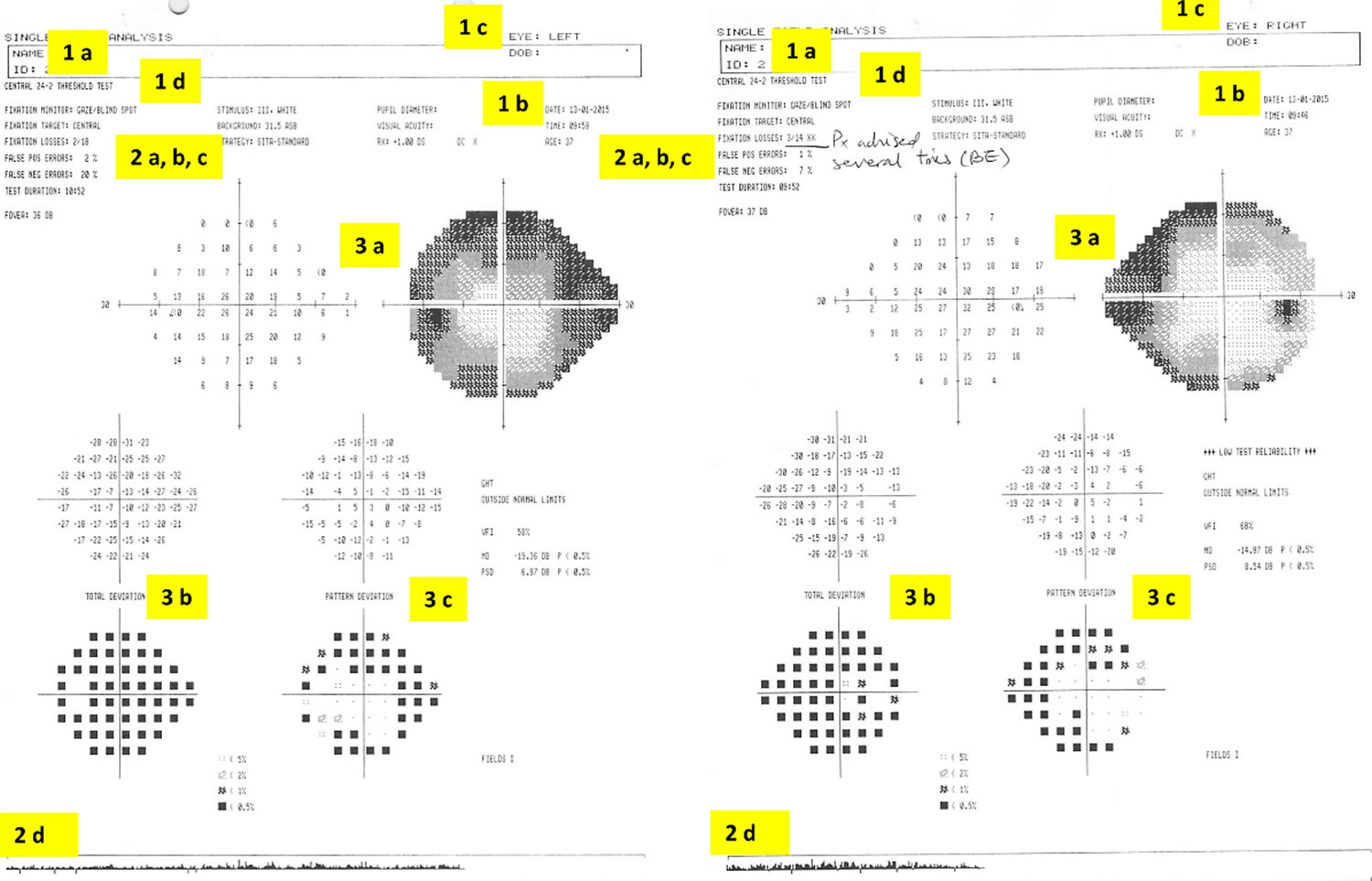
Footnote: Interpreting the Humphrey visual field. The charts are viewed from the perspective of the patient looking into the test bowl, as if patient is looking into the paper. Suggested checklist to systematically review Humphrey visual fields (see text for details):

1. Is this the correct test?

• A. Patient name and identification number
• B. Date of test
• C. Left or right eye?
• D. Test performed degree of visual angle tested test protocol: threshold or screening

2. Can I rely on this test?

• A. False-positive errors
• B. False-negative errors
• C. Fixation-loss index
• D. Gaze-tracking graph

3. Is the test normal?

• A. Visual sensitivity map
• B. Total deviation map
• C. Pattern deviation map

This patient’s test was unreliable: high fixation loss index (and comment from technician, ‘patient advised several times for both eyes’ (suggesting poor compliance), gaze-tracking graph also showed eye movements (indicated by upward spike from baseline) and high false-negative errors, up to 20% in the left eye. The grey scale visual sensitivity map suggests a ‘clover leaf’ type pattern. This provided the impression that the patient had difficulty with the Humphrey test itself. Clinical examination including visual acuity, color vision, pupillary examination and visual field to confrontation to red pin was normal. The patient’s Goldmann visual field test was normal (Figure 4).

Visual field test results

Features of glaucomatous visual field defects

Visual field loss can be diffuse (as with cataract or corneal opacification), but more commonly there are isolated defects. The visual field defects associated with glaucoma appear to be fairly non-specific, although typical loss fits with the arrangement of the retinal ganglion cell axons within the retinal nerve fibre layer of the retina.

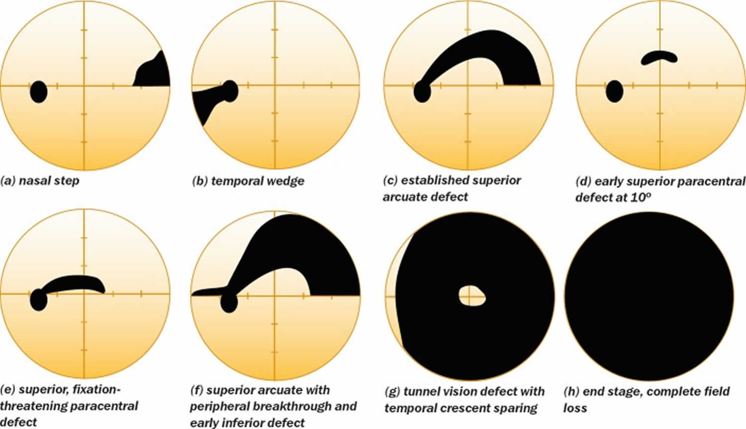
Relatively specific glaucomatous visual field defects (see Figure 7 for examples) include:

1. a nasal step defect obeying the horizontal meridian
2. a temporal wedge defect
3. the classic arcuate defect, which is a comma-shaped extension of the blind spot
4. a paracentral defect 10–20° from the blind spot
5. an arcuate defect with peripheral breakthrough
6. generalized constriction (tunnel vision)
7. temporal-sparing severe visual field loss
8. total loss of field.

Figure 7. Glaucomatous visual field defects

[Source ⁷ ]

The differential diagnosis for visual field loss similar to that seen with glaucoma includes:

• optic nerve head drusen
• retrobulbar optic neuritis
• tilted optic nerve
• anterior ischemic optic neuropathy
• neurological field defects (especially bitemporal homonymous hemianopia)
• other rare optic nerve disorders
• focal retinal disease
• visual field artefacts.

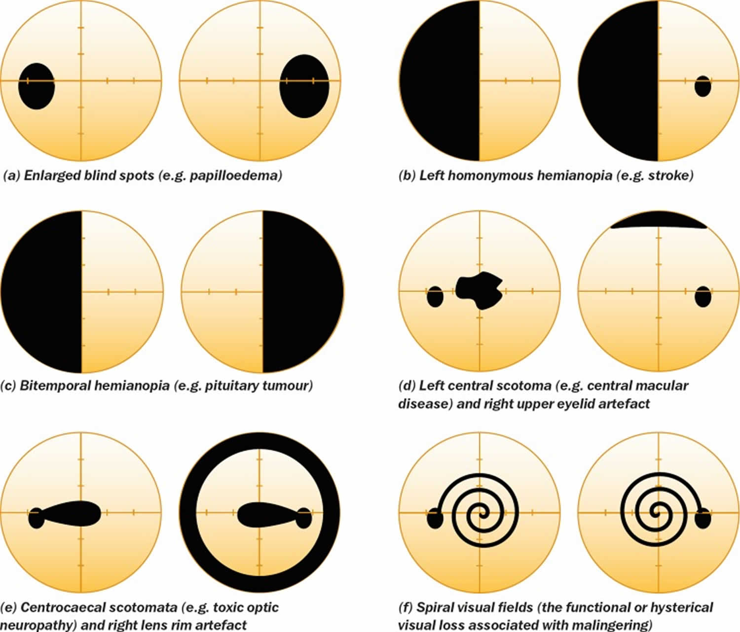
Some non-glaucomatous visual field defects are shown in Figure 8.

Figure 8. Non-glaucomatous visual field defects

[Source ⁷ ] References

1. Johnson CA, Wall M. The Visual Field. Chapter 35 in Adler’s Physiology of the Eye, 11th ed (Levin, Nilsson, Ver Hoeve, Wu, Kaufman and Alm, eds), 2011, pp 655-676.
2. Anderson DR, Patella VM. Automated Static Perimetry. 2nd edition, St Louis, Mosby, 1998.
3. Hart WM Jr, Burde RM. Three-dimensional topography of the central visual field. Sparing of foveal sensitivity in macular disease. Ophthalmol. 1983; 90(8):1028-38.
4. Armaly MF. The size and location of the normal blind spot. Arch Ophthalmol. 1969; 81(2):192-201.
5. Sample PA, Dannheim F, Artes P, Dietzsch J, Henson D, Johnson CA, Ng M, Schiefer U, Wall M. Imaging and Perimetry Society Standards and Guidelines. Optom Vis Sci 2011;88:4-7
6. Heijl A, Patella VM, Bengtsoon B. The field analyzer primer:effective perimetry. 2012, Carl Zeiss Meditec
7. Broadway DC. Visual field testing for glaucoma – a practical guide. Community Eye Health. 2012;25(79-80):66–70. https://www.ncbi.nlm.nih.gov/pmc/articles/PMC3588129/